DATE July 17, 2023 LAST EDITED May 31, 2026

• on-device ai
• quantization
• transformer

Sub-3bit transformers for fast on-device translation

How binary-code-based quantization and BiQGEMM enable sub-3-bit Transformer inference on mobile devices. Originally written in 2023 based on a 2020 paper.

Code: github.com/insoochung/transformer_bcq

TL;DR

This article showcases the benefits of BCQ: 1. BCQ’s ability to achieve extremely low bit quantization, and 2. readily available mixed precision matmul scheme BiQGEMM allowing fast on-device inference.

For reference, Chung & Kim et al. (2020) demonstrated 3.5x speedup, 8.3x runtime memory reduction, and 11.8x model size compression with sub-3bit transformers on the on-device translation task while preserving BLEU scores.

Models are larger than ever

Models continue to grow in size as performance improves with scale. However, this size expansion poses a challenge for the general public, as it becomes increasingly difficult to harness the power of these machine learning models on personal devices.

Using cloud-hosted ML products can create privacy tradeoffs.

Additionally, the cost of training large language models poses significant challenges for small companies, creating barriers to entry and concentrating power within the industry.

Consequently, this concentration of power among tech giants and well-funded corporations can narrow who gets to experiment at the frontier, limits access to state-of-the-art language models, and hampers the ability of smaller companies to offer unique features and capabilities.

In the context of neural network compression, the significance of compression techniques becomes increasingly crucial. However, neural network compression is a multi-objective optimization problem that aims to reduce inference latency, runtime memory usage, and model size while maintaining accuracy. Among these techniques, binary-code-based quantization is one useful point in this tradeoff space.

This method proves particularly valuable when applied to transformers, which serve as the foundational element for AI advancements across various domains.

In this article, our focus centers on highlighting the importance of binary-code-based quantization as a means to optimize neural networks, specifically transformers.

Sub 3-bit transformer quantization

Binary-code-based quantization (BCQ) emerges as a highly effective quantization method specifically designed for transformers. Chung & Kim et al. (2020) demonstrated its potential by achieving sub 3-bit quantization for transformer models in multiple translation tasks, with negligible loss in BLEU score, within -0.5 BLEU across three translation tasks. Furthermore, BCQ also delivers a 3.5x speedup and an 8.3x reduction in runtime memory footprint compared to full precision 32-bit models.

BCQ offers distinct advantages over the well-known uniform 8-bit quantization:

1. Low bit weights can be efficiently multiplied with full precision activation, resulting in substantial speed gains with minimal impact on task performance. In contrast, uniform quantization requires activation quantization for quantized inference, often leading to higher quantization errors and latency overhead.
2. BCQ enables extremely low bit quantization, as empirically demonstrated in Chung & Kim et al. (2020).

In the following content, we will discuss why BCQ is capable of achieving these outcomes through its unique advantages of efficient mixed precision multiplication, resulting in significant speed gains with minimal impact on task performance, as well as its ability to enable extremely low bit quantization.

High inference overhead of uniform 8-bit quantization

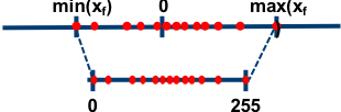
Before we talk about BCQ, it is crucial to shed light on the overheads associated with uniform quantization. Uniform quantization entails the mapping of 32-bit full precision weights to 8-bit integer weights. This process involves several steps for each weight matrix: determining the min-max value range, followed by mapping each FP value within the matrix to a corresponding value ranging from 0 to 255, or sometimes -127 to 127.

The objective is to ensure that the smallest value is mapped to 0 and the largest value is mapped to 255.

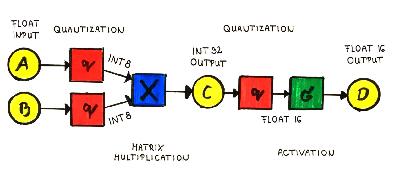
While the process of uniform quantization is straightforward and effective for various neural networks, the predicament arises during the inference phase. The crux of the issue lies in the absence of a known effective scheme for multiplying INT8 weights with FP32 activation values. To perform matrix multiplication between the quantized weights and float input values, one of two approaches must be taken.

1. Runtime weight dequantization
2. Quantized matmul by quantizing FP32 activation to INT8

Runtime weight dequantization involves dequantizing the quantized weight values to FP32. Since the matrix multiplication is performed between dequantized FP32 weights and FP32 activation values, no speed improvement can be expected.

Quantized matmul by quantizing FP32 activation to INT8 introduces notable problems. First, quantizing the FP32 activation introduces additional noise to the overall quantization scheme, potentially leading to further degradation in task performance. Secondly, the matmul operation between INT8 weights and activation values results in an INT32 output matrix. To ensure compatibility, the output range should be pre-established, which often involves approximations that may not be fully accurate. See Bhandare et al. (2019) for an example of this direction in Transformer NMT.

Additionally, the INT32 result must be converted back to INT8 to be passed on to the next layer, typically involving a two-stage data conversion process: INT32 -> FP32, or FP16, -> INT8, further increasing overall latency.

The lack of a direct “as-is” multiplication scheme between INT8 weights and FP activation values forces uniform quantization’s inference to suffer from high memory and latency overhead and additional quantization noise.

Furthermore, studies have highlighted the varying significance of computations in full precision. As a consequence, achieving an optimal trade-off between accuracy and latency often requires a combination of full precision and quantized operations. Uniform quantization’s lack of flexible mixed precision matmul approach poses a challenge in this regard, limiting the ability to strike the desired balance.

Binary code based quantization

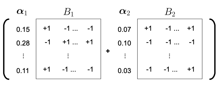
The implementation of BCQ involves the conversion of FP weights into a set of 1-bit weights, represented by B matrices, and corresponding FP scale parameters grouped in alpha vectors. Notably, each parameter in the alpha vector corresponds to a row of the original FP weight matrix W. For instance, when applying a 2-bit BCQ to an FP matrix with shape m x n, we obtain two m x n 1-bit matrices B1 and B2, accompanied by two FP vectors alpha1 and alpha2 of length m.

Now, let’s discuss how we can transform W into B’s and alpha’s. There exist several methods to approximate the B matrices and alpha vectors, and here we introduce the greedy approximation scheme:

1. Initialize the residual matrix R to be equal to the original FP weight matrix W.
2. Determine the parameters of the Bk matrix by assigning either +1 or -1 based on the sign of the corresponding value in W.
3. Compute the values in alphak such that it minimizes the difference between R and alphak * B, where each parameter in alpha is multiplied to a row in B.
4. Update R by subtracting the product of B and alpha: R = R - alphak * Bk.
5. Repeat steps 2-4 n times for n-bit BCQ.

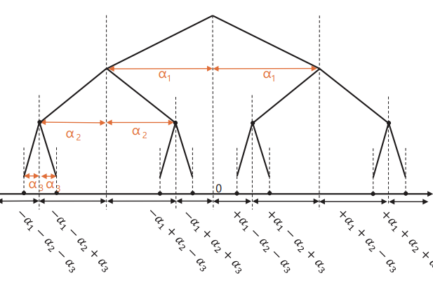
Conversely, the dequantization process would be:

$$W' = \alpha_1 B_1 + \alpha_2 B_2 + \cdots + \alpha_k B_k$$

Efficient “as-is” matmul between binary weights and FP values

One advantage of BCQ is its efficient mixed-precision multiplication between quantized weights and FP activation values during inference. This process eliminates the need for runtime data conversion, thereby avoiding redundant overhead and the introduction of additional errors.

The key to achieving this seamless operation lies in BiQGEMM, a dynamic programming-based matrix multiplication approach that enables a seamless mixed precision approach. To understand the inner workings of BiQGEMM, consider the matrix multiplication between the quantized weights $W'$ and the FP-valued vector $x$, which can be represented as follows:

$$y = W'x = \alpha_1(B_1 \cdot x) + \alpha_2(B_2 \cdot x) + \cdots + \alpha_k(B_k \cdot x)$$

As discussed, the elements in $B$ are either 1 or -1, indicating that the output elements of $B \cdot x$ are always derived from the set of all possible add-subtract combinations of $x$‘s elements. Exploiting this property, we can 1. divide the $B \cdot x$ workload into sub-regions, and 2. precompute all possible outcomes of $B' \cdot x'$ per sub-region and reuse these values for efficient mixed precision matrix multiplication.

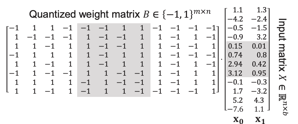
Consider the hypothetical scenario presented in Figure 7, where the B matrix has dimensions of 12 x 8, and x is a vector consisting of 12 elements. To obtain the resulting vector y, with a length of 8, each element in the i-th row of B is multiplied by the corresponding element in the x vector. To optimize the computation, we can divide x and B into three segments, as indicated by the white and gray highlights in the figure.

This allows us to express y as the sum of three sub-problems: B’ dot x’, B” dot x”, and B''' dot x'''. By addressing these sub-problems, each involving a subregion of x and B, we can efficiently perform the original matrix multiplication using 3 * 2^4 pre-computed intermediate values.

Once all the intermediate values are computed, the computation of B dot x simplifies to a sequence of indexing and addition operations, exploiting the reuse of the same intermediate values multiple times for improved efficiency. Furthermore, the subsequent multiplication between scale vectors and B dot x is straightforward.

The principles we discussed for vector-matrix level matrix multiplication using BiQGEMM can be seamlessly extended to matrix-matrix multiplication scenarios. Moreover, BiQGEMM incorporates additional optimizations, such as reusing negated pre-computation values to reduce computational overhead by half and utilizing bit-packed indices for faster indexing of pre-computed values. For more detailed explanations of these optimizations, refer to the original paper.

As demonstrated by Chung & Kim et al. (2020), BiQGEMM’s efficient matrix multiplication method provides fast and efficient inference, rendering BCQ a highly beneficial approach for on-device transformer use cases, such as translation. Also, the ability to perform matrix multiplication between quantized weights and FP activation values allows BCQ to have a flexible approach, such as only quantizing layers that are not subject to large loss in task performance when perturbed.

Recovering from high quantization error

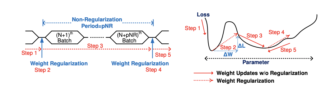
When mapping FP values to extremely low-bit datatypes, such as sub-3 bits, significant quantization errors are likely to occur, resulting in a sharp decline in task performance. To address this issue, an effective approach is to incorporate a period of non-regularization, or pNR. By considering quantization as a form of weight regularization, we recognize that it limits the potential range of model weights within the loss surface.

Introducing pNR allows the target model to freely explore the loss space, occasionally enforcing the quantization constraint to strike a balance between quantization requirements and optimal task performance. For instance, in the case of transformers, a simple implementation could involve training the model with FP weights and applying quantization every 1000 batches to evaluate its performance. The figure below illustrates the training process with pNR.

Experiments show pNR constants ranging from 500 to 2000 yielded satisfactory results for transformers, with little variation between them. The use of a large pNR value implies that the quantization overhead is rarely incurred, resulting in only a marginal increase in overall training time.

By integrating a period of non-regularization into the training process, the adverse effects of severe quantization errors can be mitigated, allowing for improved task performance while minimizing the impact on training efficiency.

Fine-grained compression approach for transformers

Fine-grained compression is essential when dealing with transformers, as compressing them presents significant challenges. These challenges arise from various factors. Firstly, different layers within a transformer exhibit varying sensitivity to compression errors. Some layers can tolerate quantization errors without a substantial impact on task performance, while others are more sensitive to such errors. Secondly, real-world applications often have highly variable word frequency distributions.

As a result, applying a uniform compression approach to all word vectors in an embedding may not yield optimal results. Lastly, compression rates and latency improvements vary across different parts of transformers. For instance, the autoregressive inference scheme requires multiple decoding steps but only a single encoding step.

Addressing these challenges, Chung and Kim (2020) propose a quantization scheme that assigns varying bit precision to different parts of the transformer. This fine-grained quantization approach can be categorized based on the level of granularity in the quantization scheme.

Block-wise scheme

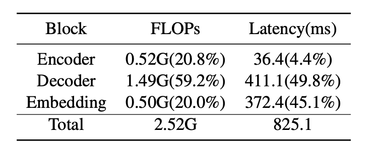
The contribution of each block in a transformer, encoder, decoder, and embedding, to the total latency is depicted in Table 1. While the encoder block demonstrates minimal overall overhead, the decoder and embedding-related functions account for the majority of the inference time. It is important to note that the actual latency overhead differs from FLOPs measurements, as factors such as parameter loading-unloading and cache utilization significantly impact overall latency.

Layer-wise scheme

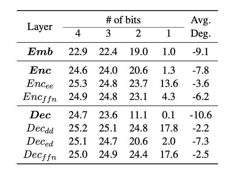
Table 2 illustrates the varying sensitivity of different layers to quantization. Certain layers exhibit higher sensitivity, resulting in a steep degradation in BLEU score when subjected to quantization errors. Taking this into consideration, Chung and Kim (2020) propose a quantization scheme that assigns a higher number of bit-precision to sensitive layers while allocating lower bit-precision to more robust layers.

In general, higher bit precision is assigned to encoder sub-layers compared to decoder sub-layers, considering the block-wise contribution to the overall latency.

Vector-wise scheme

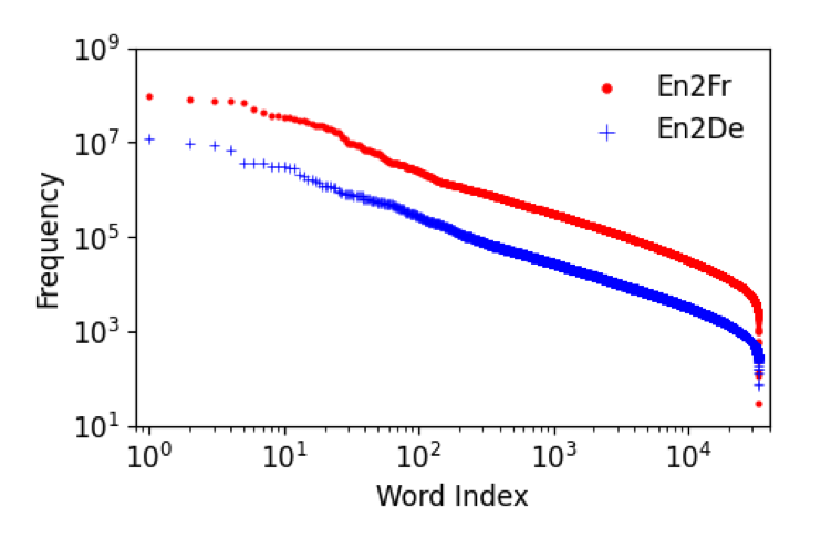
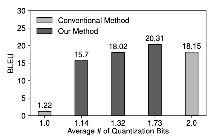
In real-world text, words exhibit a power law frequency distribution, where certain words are highly frequent while others are rarely encountered. Building upon this observation, Chung and Kim (2020) propose a vector-wise scheme that assigns varying numbers of bits based on word frequency. Specifically, a group of the most frequent words is allocated a higher number of bits, such as 4 bits, while subsequent groups receive progressively fewer bits, such as 3, 2, and 1 bits.

This fine-grained approach enables efficient compression of the embedding block while preserving accuracy. Notably, Figure 10 demonstrates that employing this fine-grained approach maintains BLEU scores more effectively at lower average bit-precision levels.

Application: on-device translation with sub-3bit transformer

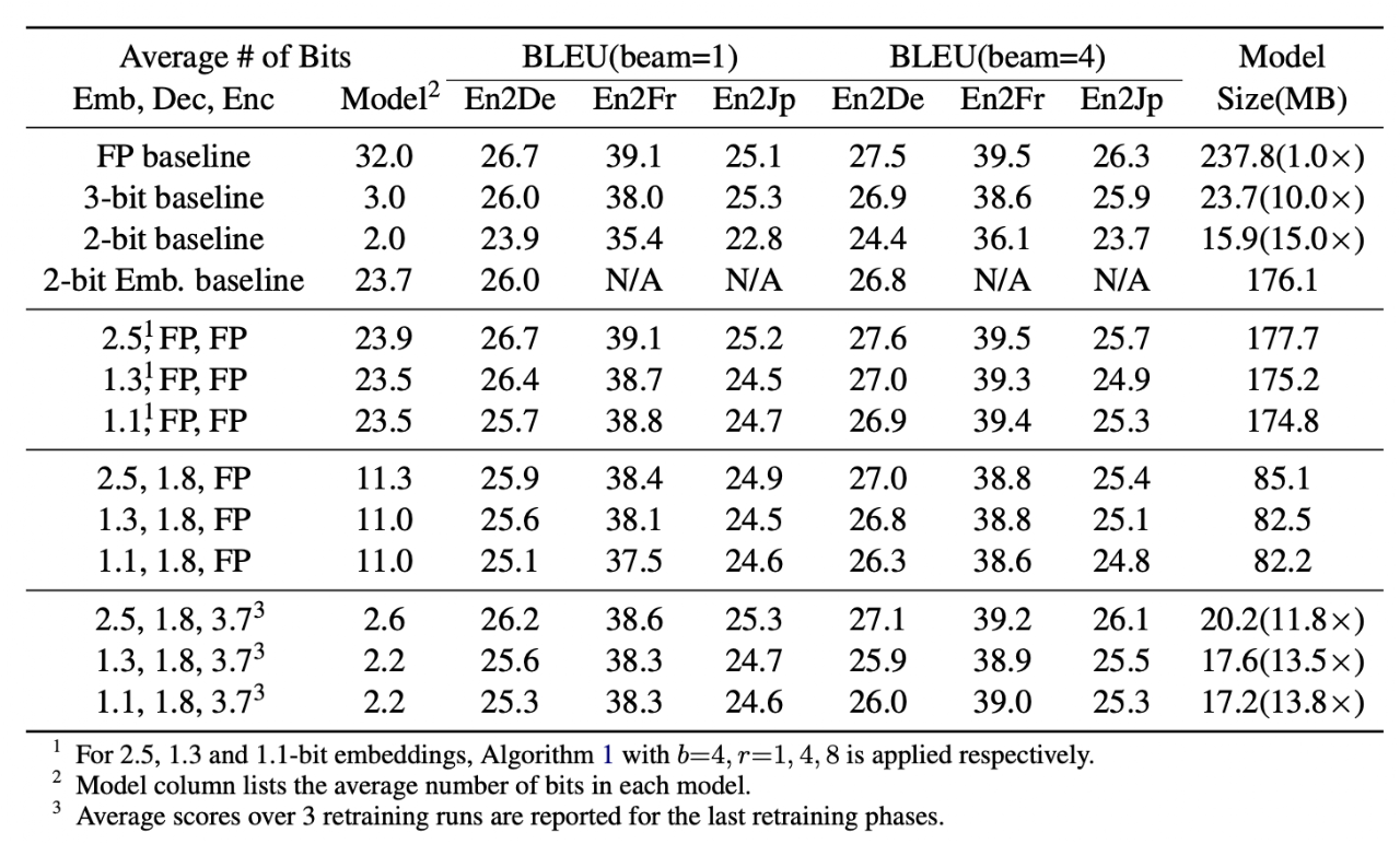
Table 3 showcases the results from Chung & Kim et al. (2020). In this research, the authors introduce a sub-3-bit transformer model. The experimental findings show that this transformer model offers benefits when applied to on-device translation tasks.

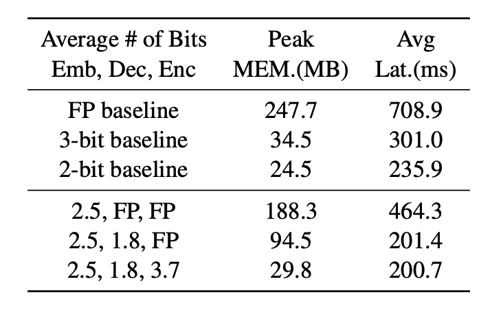
The 2.7-bit transformer implementation brings substantial improvements. It accelerates inference by 3.5x, achieves an 8.3x runtime memory compression, and reduces model size by 11.8x, improving on-device translation efficiency.

Conclusion

This article explores the possibilities and benefits of binary code-based quantization. BCQ shines in its ability to facilitate extremely low bit quantization and offers a flexible mixed precision matrix multiplication scheme between binary weights and full precision activation values. Later work, such as Park et al. (2022) and Kwon et al. (2022), explores related BCQ-style ideas for larger generative models.

P.S. Implementation of BCQ is not as complex as it reads. This repository demonstrates the implementation of 3-bit BCQ on a transformer model for a translation task. It may give you some insight into how you can apply BCQ to your own project. Hope this helps.

References

• Chung, I.*, Kim, B.*, Choi, Y., Kwon, S. J., Jeon, Y., Park, B., Sangha Kim, and Dongsoo Lee. 2020. Extremely Low Bit Transformer Quantization for On-Device Neural Machine Translation. Findings of EMNLP 2020.
• Bhandare, A., Sripathi, V., Karkada, M., Menon, H., Choi, K., Datta, K., and Saletore, V. 2019. Efficient 8-bit quantization of transformer neural machine language translation model.
• Jeon, Y.*, Park, B.*, Kwon, S. J., Kim, B., Yun, J., and Lee, D. 2020. BiQGEMM: matrix multiplication with lookup table for binary-coding-based quantized DNNs.
• Lee, D., Kwon, S. J., Kim, B., Jeon, Y., Park, B., Yun, J., and Wei, G. 2020. Decoupling Weight Regularization from Batch Size for Model Compression.
• Park, G.*, Park, B.*, Kwon, S. J., Kim, B., Lee, Y., and Lee, D. 2022. nuQmm: Quantized matmul for efficient inference of large-scale generative language models.
• Kwon, S. J., Kim, J., Bae, J., Yoo, K. M., Kim, J. H., Park, B., and Lee, D. 2022. AlphaTuning: Quantization-Aware Parameter-Efficient Adaptation of Large-Scale Pre-Trained Language Models.

* Equal contribution.