A recent history of range, resolution, and outlier handling in low-bit LLMs.
How modern LLM quantization methods spend their limited numeric budget by splitting, scaling, migrating, and rotating outliers.
1. Introduction: why LLM quantization has an outlier problem
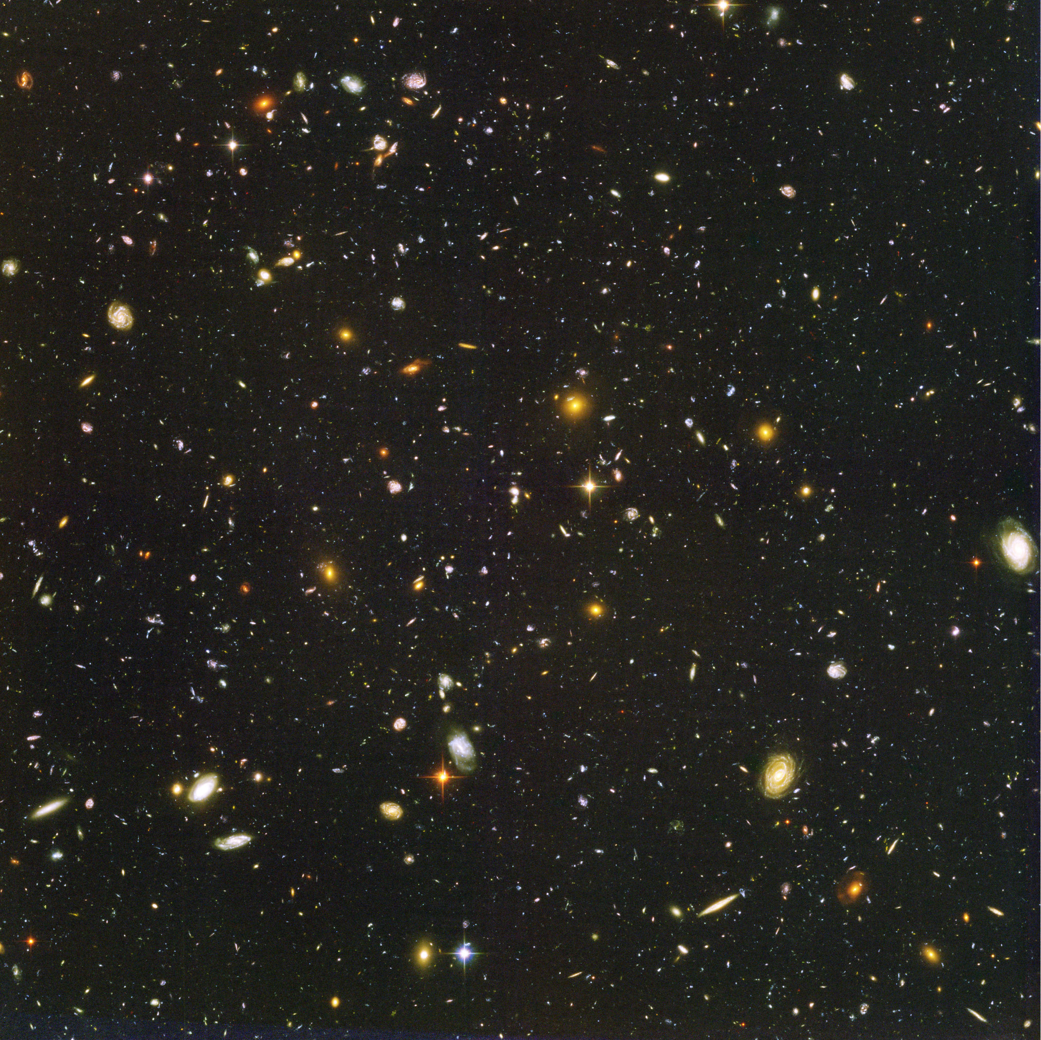
Figure 1. The Hubble Ultra Deep Field. Source: NASA Hubble
In the Hubble Ultra Deep Field photo, in the black patches between the visible galaxies, there may still be fainter, farther sources below the image’s display threshold. What we see is shaped by dynamic range: visible galaxies occupy a wide part of the rendering range, while weaker sources are compressed toward relative nothingness, indistinguishable from the black background. The image has to spend its visible range on both the bright objects and the faint background structure. When the image tries to render a wide visible range, small differences near the dark end become harder to see.I realize this is not a perfect scientific analogy. The HUDF is a carefully processed long-exposure image that actually reveals the farther sources not usually seen. But it is beautiful, and it gives us a useful way to start thinking about range.
LLM tensors have the same kind of range problem. A weight matrix, activation tensor, or KV cache is a collection of numbers, and each number has to be stored with a finite bit budget. Full precision formats such as FP32 spend many bits to cover both a wide numeric range and small differences within that range. Low-bit quantization deliberately spends far fewer. If a few outlier values stretch the range, more of the budget is spent covering the extremes, and the ordinary values in the middle collapse into coarser steps.
1.1 Quantization basics
Consider a tensor of full-precision values, . Quantization replaces those high-precision values with lower-precision codes so the model can use less memory, move less data, and often run faster on hardware that supports low-precision arithmetic. The details vary, but the basic operation is simple: choose a numeric range, divide it into buckets, and store each value as the ID of the nearest bucket.
For now, consider uniform 8-bit quantization. In the simplest min/max version, the quantizer stores a lower and upper bound for as shared full-precision metadata. Given and , the 256 integer IDs from 0 to 255 correspond to evenly spaced real-valued points across that stored range. Each tensor value is then stored as the ID of the nearest point.In practice, quantized tensors usually carry a small amount of auxiliary metadata, such as scale, zero-point, min/max, or group-wise statistics. These values may be shared per tensor, per channel, per column, or per group. This means “k-bit quantization” often uses slightly more than k bits per value on average: for example, a nominal 2-bit format might be closer to 2.1 bits once metadata is counted.
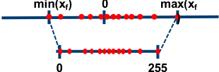

Figure 2 illustrates the mapping between quantized values and full precision values, while Figure 3 is the actual quantization equation used to map a full precision value () to the bucket ID ().
This 8-bit recipe was a strong practical baseline before the LLM era. Both CNN-based vision models and RNN-based language models were shown to preserve competitive accuracy with this simple 8-bit scheme.
1.2 LLM quantization’s outlier problem
Large transformers, the building blocks of modern LLMs, turned out to be harder to quantize than the pre-LLM CNN and RNN use cases. LLM.int8() showed that standard 8-bit baselines begin to degrade at multi-billion-parameter scale, especially after large-magnitude outlier features emerge.
The culprit is not that every value becomes hard to compress. Rather, a small number of activation feature dimensions can become much larger than the rest, stretching the quantization range and increasing the error for ordinary values. The demo below shows the same pressure in a toy tensor. The top row contains the floating-point values in their original real-valued range. The bottom row shows where those values land after min/max uniform quantization.
Start with the Gaussian distribution. Most values live near zero, so the quantizer can spend its buckets where the data actually is. Even with the values quantized to 3-bit or 2-bit, the center is coarse but still recognizable. The mean error, , stays relatively low.
Now switch to the LLM-like distribution, which is still mostly Gaussian but has occasional large outliers. The min/max range expands to include those outliers, so with quantization, many buckets are spent covering the empty gap between the dense middle and the tail. When the bit budget drops below 4 bits, that waste becomes expensive. At 2-bit or 1-bit, many ordinary values collapse into the same few bucket IDs, considerably increasing the quantization error. That is the outlier problem in one picture: low-bit quantization has very few buckets, and outliers decide where those buckets go.
This is not just a toy failure mode. The same pattern keeps reappearing across LLM quantization papers, under slightly different names and on slightly different tensor surfaces. LLM.int8() names the phenomenon emergent outlier features. SmoothQuant, AWQ, QuIP, QuaRot, and SpinQuant all run into a version of the same issue and propose different ways to make low-bit quantization survive it.
The details differ, but the recurring question is simple: when most values are easy to compress and a few values are not, what should the quantizer do with the few? A large branch of recent LLM quantization work revolves around this question: how should a limited bit budget be split between covering range and preserving resolution?
2. Background
2.1 Why PTQ became the operating default
Simple low-bit quantization fails when outliers stretch the range: the number of buckets is fixed, but the range those buckets must cover is not. There are methods to alleviate this effect and have the model cope better with quantization noise.
- Post training quantization (PTQ) starts from an existing checkpoint and tries to compress it after the fact. Methods such as GPTQ use calibration data, weight statistics, activation statistics, or local reconstruction objectives to choose a quantized representation with minimal additional compute.
- Quantization aware training (QAT) is a more costly but powerful alternative. QAT trains or fine-tunes the model while simulating the target quantized format. The model sees rounding, clipping, and bucket noise during optimization, so the weights can adapt to the low-precision representation before deployment. That adaptation can make QAT the stronger answer when the target bit-width gets extremely low; for example, EfficientQAT reports strong 2-bit and 3-bit results across llama models.
But QAT has a cost: (1) training or fine-tuning compute, (2) risk of behavior drift from the original checkpoint. For small or purpose-trained models, compute price can be reasonable. For large LLM checkpoints, it is much harder to ignore. Also, a small behavior shift can disturb trained objectives (e.g. instruction tuning, safety tuning, and serving-specific patches). To summarize:
| Method | When | Benefit | Caveat |
|---|---|---|---|
| PTQ | After the checkpoint exists | Much cheaper to apply to existing checkpoints - focus of this note | Less powerful than QAT when the bit budget gets extremely small |
| QAT | During training or fine-tuning | The model can adapt to quantization noise, so it can be stronger at very low bits | Training compute, representative data, and behavior drift |
In practice, that cost pushes much of LLM quantization research toward PTQ. As a rough arXiv title/abstract proxy from 2021-01-01 to 2026-06-12, “post-training quantization” AND “large language model” returned 258 results, while “quantization-aware training” AND “large language model” returned 51. Acronym queries showed a similar gap: PTQ AND “large language model” AND quantization returned 165, while QAT AND “large language model” AND quantization returned 35.This is only a rough search proxy, not a bibliometric claim. For the rest of this note, I will focus on PTQ: methods that start with an existing checkpoint and try to make it cheaper to serve.
2.2 Quantization is not one surface
“Quantization” is a broad word. In LLM deployment, it usually means one of three surfaces.
- Surface 1 - weight: the activations can still flow through the model in higher precision. This is the surface for methods like GPTQ and AWQ.
- Surface 2 - weight+activation: both weights and activations are quantized. This is usually done to take advantage of fast integer multiply-add schemes, as in SmoothQuant.
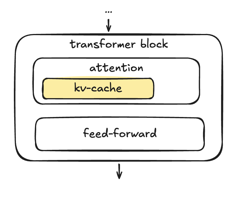
- Surface 3 - KV-cache: in autoregressive transformer models, previous tokens create key/value vectors that can be reused for subsequent tokens. Naturally these states are cached, but as context gets longer, the memory requirement can be prohibitive. This is another important area of concern, especially with recent agent developments; TurboQuant is one recent example.
This note will cover research that spans across these surfaces, but the focus will be the same: how outliers are handled when both range and resolution are scarce.
3. Quantization’s battle against outliers
Section 1 framed low-bit quantization as a range-resolution tradeoff: the buckets are fixed, but outliers can stretch the range those buckets must cover. Section 2 gave the background: PTQ is the practical default, and quantization can target different tensor surfaces. Now we can ask the main question: when a few values stretch the range, what should the quantizer do with them?
Recent methods answer that question in a few recurring ways. Split the outliers out. Move the difficulty somewhere else. Scale around the sensitive values. Or rotate the space so the quantization error hurts less. Let’s dig in deeper at each method.
3.1 Split them out
LLM.int8() gives the most literal answer: keep most of the computation in int8, but route the outlier feature dimensions through a higher-precision path.
The paper’s key empirical observation is that the outliers are not spread randomly across the tensor. Around the multi-billion-parameter scale, large activation values begin to appear systematically in a tiny number of feature dimensions. They are sparse as a fraction of all values, but important for model behavior. That matters because a normal int8 matrix multiply has one problem: a few huge activation channels can stretch the quantization range for the whole operation.
LLM.int8() handles this by decomposing the matrix multiply. The ordinary feature dimensions go through vector-wise int8 quantization, with separate normalization constants for the inner products, and then int8 matrix multiplication. The outlier dimensions are separated and multiplied in higher precision, then added back into the output. In other words, the outlier stays an outlier. The method just refuses to make every value pay the same price for it.
In matrix form, the split is roughly . The bulk term runs through the int8 path. The outlier term stays small enough to handle separately in higher precision.
This made 8-bit inference viable for very large models: the paper reports loading and converting 16/32-bit checkpoints up to 175B parameters to int8 without performance degradation, while still doing more than 99.9% of the value multiplications in 8-bit. The tradeoff is systems complexity. If the outlier gets its own path, the kernel gets a side path too. The system now has to track outlier channels, route them separately, execute a small higher-precision multiply, and fuse the result back into the main output.
3.2 Move the difficulty into weights
SmoothQuant starts from a different observation: activations are often harder to quantize than weights. Instead of splitting activation outliers out, it uses an equivalent scaling transform to move some of the activation difficulty into the weights before inference.
The method works per hidden channel. Suppose a linear layer computes , where each column of and matching row of share one channel dimension. SmoothQuant inserts a diagonal scale matrix and rewrites the same computation as . For channel , the activation column is divided by , and the matching weight row is multiplied by the same .
Nothing about the full-precision function changes. What changes is the quantization surface. Large activation channels become smaller before runtime activation quantization, while the compensating larger weights can be quantized offline.
The knob is how much difficulty to migrate. SmoothQuant uses one global migration hyperparameter, , but the actual scale is still per-channel: . Larger puts more emphasis on smoothing the activation side; smaller leaves more of the burden on activations and keeps weights more normalized. The outlier is not removed; its pressure is moved.
The improvement over LLM.int8() is that there is no separate outlier matmul to route and fuse. SmoothQuant keeps one ordinary runtime matrix multiply and makes W8A8 inference practical by making activations less hostile to int8 kernels. The authors report INT8 weights and activations for all matrix multiplications across OPT, BLOOM, GLM, MT-NLG, Llama, Falcon, Mistral, and Mixtral-style models, with up to 1.56× speedup and 2× memory reduction under negligible accuracy loss. They also show serving a 530B-parameter model within a single node.
3.3 Protect what matters with scales
AWQ is weight-only PTQ, but it is activation-aware. It asks which weights matter for the observed activations and protects a small salient subset through scaling.
The central point is that weight magnitude alone is not a reliable guide to importance. A modest-looking weight can matter a lot if it is repeatedly hit by large activations, while a large weight can matter less if the activation channel is usually quiet. AWQ therefore collects activation statistics offline and uses them to identify salient weight channels. It does not backpropagate through the model or reconstruct layer outputs during this step; the calibration set tells it which channels are sensitive, not how to retrain them.
The naive way to protect salient weights would be mixed precision: keep the important weights in FP16 and quantize the rest. AWQ instead tries to get the same benefit in a hardware-friendly uniform weight format. For a selected channel , it scales the weight row before quantization, , then compensates with the matching activation column, . The full-precision product is still equivalent, but the quantizer sees a larger salient weight row before rounding.
This is the scale answer, but it is different from SmoothQuant. SmoothQuant moves activation outlier range into weights so W8A8 can work. AWQ is weight-only, so activations can remain high precision at runtime. The activation samples are used for a different job: they tell the weight quantizer which channels deserve more numeric care.
The improvement is that AWQ gets much of the benefit of protecting sensitive weights without introducing a mixed-precision runtime path. Only a tiny protected subset can carry a lot of the model’s sensitivity. The paper reports that protecting about 1% of salient weights can greatly reduce quantization error, and shows strong low-bit weight-only quantization across language, code, math, instruction-tuned, and multimodal LLMs. With TinyChat, its 4-bit deployment path reports more than 3× speedup over a HuggingFace FP16 baseline on desktop and mobile GPUs.
3.4 Rotate the space
If the outlier is partly a coordinate-system problem, rotate the coordinate system.
The basic identity is for an orthogonal rotation . The full-precision function is unchanged. The coordinates seen by the quantizer are not.
QuIP frames quantization as easier when weights and Hessian directions are incoherent: values become more even in magnitude, and important rounding directions are less aligned with coordinate axes. The method combines adaptive rounding, which minimizes a quadratic proxy for the weight error, with pre- and post-processing by random orthogonal matrices. The goal is not only to reduce the largest weight values, but to make the quantization problem less axis-aligned. That was enough to make two-bit weight quantization produce viable LLM results where straightforward low-bit rounding was much more fragile.
QuaRot pushes the rotation idea into the full inference graph. It applies mathematically equivalent rotations at places where the transformer computation is invariant, so the full-precision model output is unchanged but hidden states and intermediate activations have fewer extreme coordinates. The paper uses this to quantize weights, activations, and KV cache to 4 bits, aiming for all matrix multiplications to run in low precision without keeping special channels in higher precision. Its headline result is a 4-bit LLaMA-2-70B model with at most 0.47 WikiText-2 perplexity loss while retaining 99% of zero-shot performance.
SpinQuant makes the rotation itself a target of optimization. Random rotations help, but some random rotations help much more than others; the paper reports up to a 13-point downstream reasoning spread between random choices. SpinQuant learns rotation matrices on a small validation set, preserving the full-precision function while searching for a basis that is friendlier to low-bit weights, activations, and KV cache. With 4-bit weights, activations, and KV cache, it narrows the LLaMA-2-7B zero-shot reasoning gap to 2.9 points from full precision, outperforming LLM-QAT and SmoothQuant in that setup.
This improves on the previous answers in a different direction. LLM.int8() splits the hard channels out. SmoothQuant moves the activation difficulty into weights. AWQ protects the weight channels that matter most. Rotation methods ask whether the channels themselves are the wrong coordinates. If the same function can be written in a less spiky basis, quantization has less axis-aligned damage to do.
The achievement is that this idea keeps scaling down the bit-width. QuIP made very low-bit weight quantization more viable by combining incoherence with adaptive rounding. QuaRot carried equivalent rotations through the transformer graph, reaching 4-bit end-to-end inference without special high-precision channels. SpinQuant keeps the same principle but learns the rotations, improving over fixed or random choices when calibration data can reveal a better basis.
3.4.1 Runtime state: TurboQuant
TurboQuant is worth mentioning because it shows the same rotation instinct on a different surface: online KV-cache vectors rather than static model weights.
During generation, the KV cache stores runtime vectors that grow with context length. TurboQuant is not just “rotate, then quantize.” It uses a data-oblivious random rotation so the coordinates of a high-dimensional vector follow a predictable concentrated distribution, then applies scalar quantizers tuned for that distribution. For attention, where inner products matter, it adds a second stage: an MSE quantizer plus a 1-bit Quantized JL residual path, so the inner-product estimate is unbiased. The full paper has the coding and proof details; here the point is simpler: a basis change can make runtime state quantizable too.
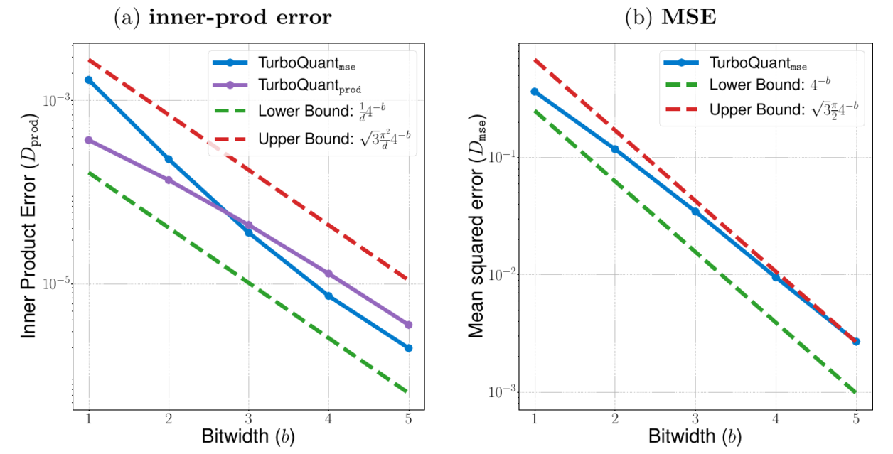
The reported result is quality neutrality around 3.5 bits per channel for KV-cache compression, with only marginal degradation around 2.5 bits per channel. The point for this note is the surface shift: the same geometry instinct can apply to runtime state, not only to fixed weights and activations.
4. Conclusion: the real target is pressure, not bits
The lesson from these papers is not that one method wins. It is that outliers decide where quantization breaks.
LLM.int8() keeps the pressure in a higher-precision side path. SmoothQuant moves it from activations into weights. AWQ protects the few weight channels that matter most. Rotation methods change the basis so the pressure is less concentrated on one coordinate. TurboQuant takes that same instinct to runtime state.
That makes these papers easier to compare if we stop asking only how many bits they use, and instead ask where they put the outlier pressure.
Table 2 is the compact version of that story:
| Method | Surface | Where the pressure goes |
|---|---|---|
| Split outLLM.int8() (2022) | Weight + activation | Route emergent outlier feature dimensions through a higher-precision path while keeping the bulk matrix multiply in int8. |
| MoveSmoothQuant (2022) | Weight + activation | Use an equivalent per-channel scaling transform to migrate activation outlier difficulty into weights before inference. |
| ProtectAWQ (2023) | Weight | Use activation statistics to find salient weights, then protect those channels with scaling instead of minimizing average error everywhere. |
| RotateQuIP (2023) | Weight | Make weights and second-order error directions more incoherent, so low-bit rounding is less dominated by axis-aligned outliers. |
| RotateQuaRot (2024) | Weight + activation | Apply rotations around the transformer so weights, activations, and cache-like states become easier to quantize together. |
| RotateSpinQuant (2024) | Weight + activation | Learn rotations that spread outlier pressure across channels before low-bit weight, activation, and KV-cache quantization. |
| RandomizeTurboQuant (2025) | KV-cache | Use online randomized rotations plus scalar quantization to make runtime vectors less sensitive to a few large coordinates. |
5. Next: inference considerations
So far, this note has treated quantization as a numerical problem: preserve behavior while spending fewer bits, and decide where the outlier pressure should go. That gives us a compressed representation, but it does not yet guarantee a faster system.
The next question is latency: can we run it faster? Weight-only methods may still dequantize into a normal GEMM path. Codebook methods can save memory but need codebook-aware kernels to turn compression into latency. W8A8 methods can line up with fast integer multiply-add paths, but only if the activation side is tame enough to quantize. That is where quantization stops being only a numerical problem and becomes an inference problem. Maybe we’ll revisit in another note 😇.